Using MOC with HATS

A HATS catalog describes a particular set of HEALPix tiles on the sphere. These tiles can alternately be described by a MOC, or Multi-Order Coverage map.

For a full introduction and reference to MOC, we suggest reading https://cds-astro.github.io/mocpy/. We use that library internally for speedy manipulation of MOCs.

This notebook will introduce you to the utilities we have found most useful for building MOCs and using those to impose a filter on catalogs.

Imports

import hats
from hats.pixel_math import region_to_moc
from hats.inspection.visualize_catalog import plot_moc

We will set the max_depth value here to something fairly small (which translates into larger area tiles) for demonstration purposes.

Later, we’ll change this to a higher value, and you’ll see finer-grained MOCs.

max_depth = 4

Basic shapes

We’ve wrapped some of the basic shapes with validating methods in the region_to_moc module, and provide a simple plotting interface.

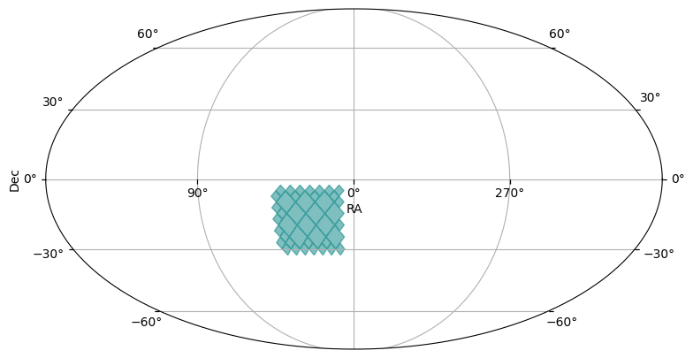
In the plots, you might see light blue diamonds with darker blue borders. Each diamond represents a single HEALPix pixel, with larger area diamonds corresponding to higher order HEALPix pixels.

box_moc = region_to_moc.box_to_moc(ra=[10, 45], dec=[-30, -5], max_depth=max_depth)
plot_moc(box_moc)

(<Figure size 900x500 with 1 Axes>, <WCSAxes: >)

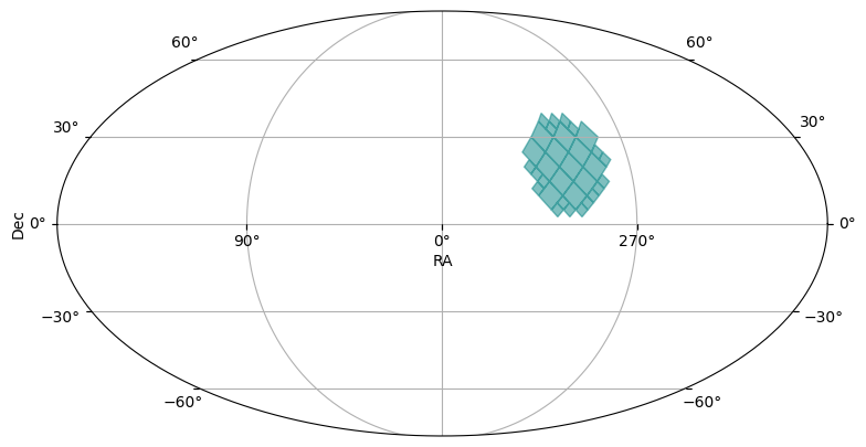
cone_moc = region_to_moc.cone_to_moc(ra=-60.3, dec=20.5, radius_arcsec=15 * 3600, max_depth=max_depth)
plot_moc(cone_moc)

(<Figure size 900x500 with 1 Axes>, <WCSAxes: >)

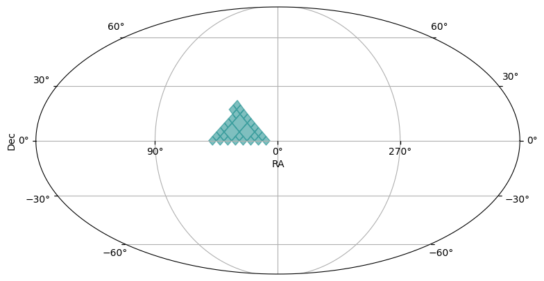
polygon_moc = region_to_moc.polygon_to_moc([(10, 0), (45, 0), (30, 18)], max_depth=max_depth)
plot_moc(polygon_moc)

(<Figure size 900x500 with 1 Axes>, <WCSAxes: >)

Operations on MOCs

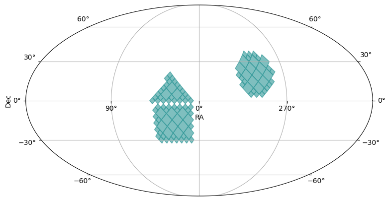
The MOCPy library provides lots of additional operations on MOC objects. Below we show an addition (or union) of the three MOCs we generated above.

Further, we take the inverse (or complement) of that union MOC, to see everything NOT represented in the first MOC.

union_moc = polygon_moc.union(cone_moc, box_moc)
plot_moc(union_moc)

(<Figure size 900x500 with 1 Axes>, <WCSAxes: >)

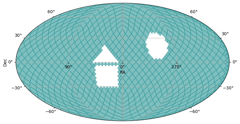
complement_union_moc = union_moc.complement()
plot_moc(complement_union_moc)

(<Figure size 900x500 with 1 Axes>, <WCSAxes: >)

Filtering a catalog with a MOC

We’ll use the union_moc we created above to perform a coarse spatial filter on the data partitions of an existing HATS catalog. This catalog is used for test and demonstration purposes, and so has a kind of silly set of partitions.

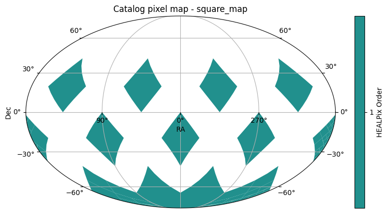
The first plot is the set of partitions, as solid order 1 HEALPix pixels.

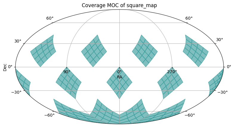
The second plot shows the MOC of the catalog, with divisions at order 4.

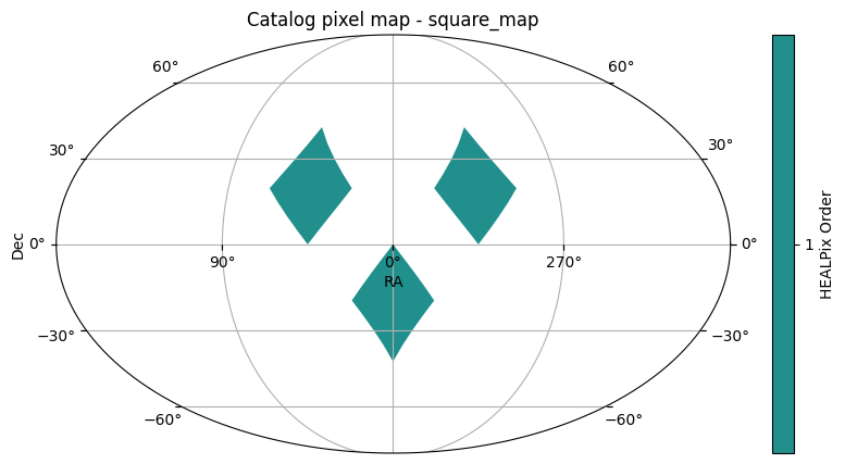
You will see in the third plot that only those pixels with some amount of overlap with the pixels of the union_moc remain in the filtered catalog.

catalog = hats.read_hats("../../tests/data/square_map")
catalog.plot_pixels()

(<Figure size 1000x500 with 2 Axes>,
 <WCSAxes: title={'center': 'Catalog pixel map - square_map'}>)

catalog.plot_moc()

(<Figure size 900x500 with 1 Axes>,
 <WCSAxes: title={'center': 'Coverage MOC of square_map'}>)

filtered_catalog = catalog.filter_by_moc(union_moc)
filtered_catalog.plot_pixels()

(<Figure size 1000x500 with 2 Axes>,
 <WCSAxes: title={'center': 'Catalog pixel map - square_map'}>)

About

Author: Melissa DeLucchi

Last updated on: August 28, 2025